投资组合分析与Fama-Macbeth回归
薛英杰 / 2022-11-27
20世纪60年代,资本资产定价模型(Capital Asset Pricing Model,CAPM)问世。在CAPM被 提出前,人们对于风险如何影响一个公司的资本成本,进而影响预期收益率并没有清晰的认 识。CAPM模型的诞生首次清晰地描绘出风险和收益率之间的关系。
根据CAPM理论,资产预期超额收益由一个一元线性模型决定:
\[ E[R_i]-R_f=\beta_i(E[R_M]-R_f) \]
其中,\(E[]\)是期望符号,\(R_i\)为某资产的收益率,\(R_f\)为无风险收益率,\(R_M\)为市场组合的收益率。式中\(\beta_i=Cov(R_i,R_M)/Var(R_M)\)刻画了该资产对市场收益的敏感程度,也被称为资产\(i\)对市场风险的暴露程度。该模型指出资产的预期超额收益率由市场组合的预期超额收益率和资产对市场风险的暴露大小决定,而市场组合也被称为市场因子。
随着大量实证研究进行,人们发现不同资产的收益率并不是由单一的市场因子决定,而是同时受其他因子的影响。以此为契机,Ross(1976)提出了著名的套利定价理论(Arbitrage Pricing Theory,APT),在CAPM的基础上做了延伸,构建了线性多因子定价模型,并假设资产\(i\)的预期超额收益由以下多元线性模型决定:
\[ E[R_i^e]=\boldsymbol{\beta_i^\prime\lambda} \]
其中,\(E[R_i^e]\)是资产\(i\)的超额收益,\(\boldsymbol{\beta_i^\prime}\)是资产\(i\)的因子暴露,\(\boldsymbol{\lambda}\)是因子预期收益。
那么,如何检验一个因素会影响资产收益呢?学者们提出了两种方法,一种是投资组合分析,另一种是Fama-Mechth回归。本文主要利用R语言介绍这两种方法在实证中如何应用。
投资组合分析
(1)单变量投资组合分析
CAPM模型表明资产的预期超额收益率由市场组合的预期超额收益率和资产对市场风险的暴露大小决定。在横截面上,市场组合的预期超额收益对所有资产都是一样的,即风险溢价在某一时间点对所有资产来说是不变的,某个资产\(i\)的超额收益取决于该资产的风险暴露,也就是说,风险暴露越大的资产预期收益越高。因此,我们可以按照市场\(\beta\)进行分组,来检验不同组合的超额收益是否有差异。
读入所有股票月度交易数据、市场收益数据和无风险收益数据,计算股票超额收益与市场超额收益。
##加载程序包
pacman::p_load(data.table,stringr,dplyr,Tushare,sandwich ,reticulate,lubridate,mongolite,future.apply,zoo,tidyr,lmtest, haven,readxl,foreign,scales,slider,furrr,tibble,ggplot2,stargazer,tidyverse,generics)

##开启Mongo数据库
system('net start MongoDB',intern = F,wait = T)
## [1] 2##读入无风险收益数据 mogFret<-mongo(collection = "DRFRet",db="IntrestRate") Retf<-mogFret$find()%>% mutate(Tradedate=str_sub(TradingDate,1,7), MRet=(1+DRFRet)^(365/12)-1)%>% group_by(Tradedate)%>% summarise(rf=mean(MRet)) ##读入市场组合数据 mogfactor<-mongo(collection = "monthlyfactorw",db="investfactor") Marketportfio<-mogfactor$find(query = '{"market":"全市场"}',fields ='{"_id":0,"Tradedate":1,"MKT":1}' ) ##读入股票数据并拼接所有数据 mogmogth<-mongo(collection = "qfqtradedatamonthly",db="stockdata") mothdata<-mogmogth$find(query='{}', fields='{"_id":0,"ts_code":1,"trade_date":1,"close":1,"pre_close":1}')%>% mutate(MRet=close/pre_close-1, trade_date=as.Date(trade_date,"%Y%m%d"), Tradedate=str_sub(trade_date,1,7))%>% merge(Marketportfio,by="Tradedate",all.x = T)%>% merge(Retf,by="Tradedate",all.x = T)%>% filter(Tradedate>="1995-01")%>% arrange(ts_code,Tradedate)%>% mutate(ret_excess=MRet-rf, mkt_excess=MKT-rf)%>% select(ts_code,Tradedate,MRet,trade_date,ret_excess,mkt_excess)%>%tibble::as_tibble()定义估计市场\(\beta\)的函数,滚动计算月度市场\(\beta\),窗口期为60个月
##定义市场Beta的估计函数 estimate_capm <- function(data, min_obs = 1) { if (nrow(data) < min_obs) { beta <- as.numeric(NA) } else { fit <- lm(ret_excess ~ mkt_excess, data = data) beta <- as.numeric(coefficients(fit)[2]) } return(beta) } ## 定义滚动估计函数 roll_capm_estimation <- function(data, months, min_obs) { data <- data |> arrange(trade_date) betas <- slide_period_vec( .x = data, .i = data$trade_date, .period = "month", .f = ~ estimate_capm(., min_obs), .before = months - 1, .complete = FALSE ) return(tibble( month = unique(data$trade_date), beta = betas )) } ## 并行计算市场beta plan(multisession, workers = availableCores()) pdat<-mothdata|> select(ts_code,trade_date,MRet,ret_excess,mkt_excess)|> nest(data=c(trade_date,MRet,ret_excess,mkt_excess)) beta_daily <- pdat|> mutate(beta_daily = future_map( data, ~ roll_capm_estimation(., months = 60, min_obs = 50) )) |> unnest(c(data,beta_daily)) |> select(ts_code,month,ret_excess,mkt_excess,beta_daily = beta) |> na.omit()构造市场\(\beta\)组合,计算组合收益
##定义组合构造函数
assign_portfolio <- function(data, var, n_portfolios) {
  breakpoints <- data |>
    summarize(breakpoint = quantile({{ var }},
      probs = seq(0, 1, length.out = n_portfolios + 1),
      na.rm = TRUE
    )) |>
    pull(breakpoint) |>
    as.numeric()

  assigned_portfolios <- data |>
    mutate(portfolio = findInterval({{ var }},
      breakpoints,
      all.inside = TRUE
    )) |>
    pull(portfolio)

  return(assigned_portfolios)
}

##计算分组收益
beta_portfolios <- beta_daily |>
  mutate(month=str_sub(month,1,7),
         beta_lag=lag(beta_daily))|>
  group_by(month) |>
  mutate(
    portfolio = assign_portfolio(
      data = cur_data(),
      var = beta_lag,
      n_portfolios = 10
    ),
    portfolio = as.factor(portfolio)
  ) |>
  group_by(portfolio, month) |>
  summarize(
    ret = mean(ret_excess),
    .groups = "drop"
  )%>%na.omit()

beta_longshort <- beta_portfolios |>
  pivot_wider(month, names_from = portfolio, values_from = ret) |>
  mutate(long_short = get("10") - get("1"))

head(beta_longshort)
## # A tibble: 6 × 12 ## month `1` `2` `3` `4` `5` `6` `7` `8` `9` ## <chr> <dbl> <dbl> <dbl> <dbl> <dbl> <dbl> <dbl> <dbl> <dbl> ## 1 1999… -0.0455 -0.0657 -0.0569 -0.0429 -0.0552 -0.0277 -0.0519 -0.0594 -0.0514 ## 2 1999… 0.0731 0.0963 0.124 0.0872 0.0982 0.118 0.119 0.131 0.156 ## 3 1999… -0.0540 -0.0457 -0.0778 -0.0506 -0.0349 -0.00433 -0.0463 -0.0253 -0.0406 ## 4 1999… 0.0913 0.107 0.111 0.106 0.0779 0.0792 0.0637 0.119 0.0256 ## 5 1999… 0.348 0.275 0.282 0.326 0.283 0.254 0.358 0.310 0.310 ## 6 1999… -0.0515 -0.0256 -0.0599 -0.0104 -0.0824 -0.106 -0.0822 -0.0912 -0.0372 ## # … with 2 more variables: `10` <dbl>, long_short <dbl>组合业绩评估
names(beta_longshort)[2:11]<-paste0("p",1:10)
mktexces<-beta_daily|>
  mutate(month=str_sub(month,1,7))|>
  select(month,mkt_excess)
timeperfomance<-beta_longshort|>
  pivot_longer(cols=2:12,names_to = "portfolio",values_to = "ret")|>
  group_by(portfolio)|>
  arrange(portfolio)|>
  left_join(mktexces,by=c("month"="month"))|>
  unique()|>
  mutate(Date=as.Date(paste0(month,"-01")))|>
  select(portfolio,Date,ret,mkt_excess)

timeperfomance|>
  filter(portfolio%in%c("p1","p10","long_short"))|>
  mutate(cumret=cumsum(ret))|>ggplot(aes(
    x=Date,
    y=cumret,
    col=portfolio,
    linetype=portfolio
  ))+geom_line()+
  labs(
    x = NULL, y = NULL, color = NULL, linetype = NULL,
    title = "Accumuated Return for Market Beta"
  )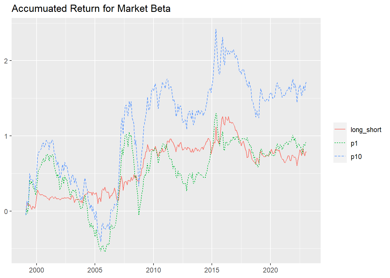
从累积收益来看,在2000年-2022年期间,高市场\(\beta\)组合(p10)的收益明显高于低市场\(\beta\)组合(p1),表明风险暴露越高的股票获得收益越高。由于多空对冲组合(long_short)是对冲掉市场风险的组合,理论上属于无风险组合,其获得的收益也相对较低,20年翻一倍,相当于年化5%的收益,略高于银行存款利率,投资股票比存钱到银行划算。
组合业绩的统计检验
##定义业绩检验函数
perforance_evaluate<-function(x,MKT){
  data<-data.frame(x,MKT)
  fit_mode<-coeftest(lm(x ~ 1+MKT, data = data), vcov = NeweyWest)
  return(c(fit_mode[1,1],fit_mode[2,1],fit_mode[1,3],fit_mode[2,3]))
}

##进行投资组合统计检验

perforance<-timeperfomance|>
  group_by(portfolio)|>
  summarise(rets=list(lm(ret ~ mkt_excess)))|>
  mutate(id=ifelse(str_detect(portfolio,"p"),
                          as.numeric(gsub("p","",portfolio)), 11))|>
  arrange(id)
## Warning in ifelse(str_detect(portfolio, "p"), as.numeric(gsub("p", "", ## portfolio)), : NAs introduced by coercionfor(i in 1:11){ assign(paste0("T",i),perforance$rets[i][[1]]) }表1:市场组合Beta超额收益
Dependent variable:
ret
(1)
(2)
(3)
(4)
(5)
(6)
(7)
(8)
(9)
(10)
(11)
mkt_excess
0.798***
0.913***
0.987***
1.010***
1.027***
1.055***
1.090***
1.113***
1.112***
1.138***
0.339***
(49.224)
(81.922)
(104.687)
(110.840)
(113.053)
(103.816)
(117.014)
(107.153)
(93.735)
(81.152)
(13.339)
Constant
-0.0002
0.003***
0.003***
0.005***
0.004***
0.005***
0.005***
0.003***
0.004***
0.002
0.002
(-0.120)
(2.606)
(3.745)
(5.840)
(4.369)
(5.570)
(5.938)
(3.325)
(3.480)
(1.249)
(0.765)
Observations
285
285
285
285
285
285
285
285
285
285
285
Adjusted R2
0.895
0.959
0.975
0.977
0.978
0.974
0.980
0.976
0.969
0.959
0.384
Note:
p<0.1; p<0.05; p<0.01
## Warning in mask$eval_all_mutate(quo): NAs introduced by coercion
虽然我们从图上看到不同市场$\beta$组合的累积收益有明显差异,但市场\(\beta\)最高组(10)和最低组(1)的统计检验并不显著,说明市场$\beta$组合捕获的资产风险很有限,也说明市场因子并不能完全解释股票收益差异。
证券市场线与\(\beta\)组合
按照资产定价模型预测,市场\(\beta\)组合应该位于证券市场线上,证券市场线的斜率等于市场风险溢价,表明在任何时候风险收益都是公平交易。
sml_capm <- lm(ret ~ 1 + beta, data = beta_portfolios_summary)$coefficients

beta_portfolios_summary |>
  mutate(portfolio=as.factor(portfolio))|>
  ggplot(aes(
    x = beta,
    y = ret,
    color = portfolio
  )) +
  geom_point() +
  geom_abline(
    intercept = 0,
    slope = mean(beta_portfolios_summary$mkt_excess),
    linetype = "solid"
  ) +
  geom_abline(
    intercept = sml_capm[1],
    slope = sml_capm[2],
    linetype = "dashed"
  ) +
  scale_y_continuous(
    labels = percent,
    limit = c(0, mean(beta_portfolios_summary$mkt_excess) * 2)
  ) +
  scale_x_continuous(limits = c(0, 2)) +
  labs(
    x = "Beta", y = "Excess return", color = "Portfolio",
    title = "Average portfolio excess returns and average beta estimates"
  )
## Warning: Removed 6 rows containing missing values (`geom_point()`).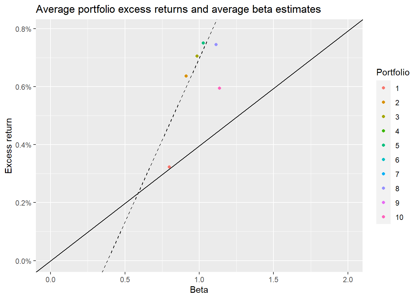
从回归结果来看,证券市场线的斜率为正,意味着高贝塔组合意味着高的市场收益。
(2) 双变量投资组合分析
在实证分析中,由于代理风险的变量之间可能存在某种相关性,比如市值和账面市值比。为了避免这种相关性对结果的影响,通常采用双变量投资组合分析,同时独立地对两种因素的分组变量进行排序,形成二维投资组合,通过检验组合收益在组合排序上是否有单调性来说明排序变量是否可以有效地捕捉到某种风险。下面以市值与账面市值比两个变量来说明双变量投资组合的应用。
##提出市值、账面市值比数据
mogbaic<-mongo(collection = "dailybasic",db="stockdata")
MandB<-mogbaic$find(query='{"trade_date":{"$gt":"19950101"}}',fields='{"_id":0,"ts_code":1,"trade_date":1,"pb":1,"total_mv":1}')%>%
  mutate(trade_date=as.Date(trade_date,"%Y%m%d"),
         Tradedate=str_sub(trade_date,1,7))%>%
  arrange(ts_code,trade_date)%>%
  group_by(ts_code,Tradedate)%>%
  summarise_all(tail,1)%>%
  mutate_at(c("pb","total_mv"),as.numeric)

mogmogth<-mongo(collection = "qfqtradedatamonthly",db="stockdata")
mothdata<-mogmogth$find(query='{"trade_date":{"$gt":"19950101"}}',
                        fields='{"_id":0,"ts_code":1,"trade_date":1,"close":1,"pre_close":1}')%>%
  mutate(MRet=close/pre_close-1,
         trade_date=as.Date(trade_date,"%Y%m%d"),
         Tradedate=str_sub(trade_date,1,7))%>%
  select(ts_code,Tradedate,MRet)%>%
  merge(MandB,by=c("ts_code","Tradedate"),all.x = T)%>%
  arrange(ts_code,Tradedate)%>%
  group_by(ts_code)%>%
  mutate(lbm=lag(1/pb),
         lm=lag(log(total_mv)))


##按市值与账面市值比划分组合
value_portfolios <- mothdata |>
  drop_na() |>
  group_by(Tradedate) |>
  mutate(
    portfolio_bm = assign_portfolio(
      data = cur_data(),
      var = lbm,
      n_portfolios = 5
    ),
    portfolio_me = assign_portfolio(
      data = cur_data(),
      var = lm,
      n_portfolios = 5
    ),
    portfolio_combined = str_c(portfolio_bm, portfolio_me)
  ) |>
  group_by(portfolio_combined,Tradedate ) |>
  summarize(
    retw = weighted.mean(MRet, lm),
    ret = mean(MRet),
    portfolio_bm = unique(portfolio_bm),
    portfolio_me = unique(portfolio_me),
    .groups = "drop"
  )|>select(-portfolio_combined)|>
  pivot_wider(names_from=c("portfolio_me","portfolio_bm"),values_from =c(retw,ret))|>
  mutate(retw_1_LH=retw_1_5-retw_1_1,
  retw_2_LH=retw_2_5-retw_2_1,
  retw_3_LH=retw_3_5-retw_3_1,
  retw_4_LH=retw_4_5-retw_4_1,
  retw_5_LH=retw_5_5-retw_5_1,
  ret_1_LH=ret_1_5-retw_1_1,
  ret_2_LH=ret_2_5-retw_2_1,
  ret_3_LH=ret_3_5-retw_3_1,
  ret_4_LH=ret_4_5-retw_4_1,
  ret_5_LH=ret_5_5-retw_5_1,
  retw_LH_1=retw_5_1-retw_1_1,
  retw_LH_2=retw_5_2-retw_1_2,
  retw_LH_3=retw_5_3-retw_1_3,
  retw_LH_4=retw_5_4-retw_1_4,
  retw_LH_5=retw_5_5-retw_1_5,
  ret_LH_1=ret_5_1-retw_1_1,
  ret_LH_2=ret_5_2-retw_1_2,
  ret_LH_3=ret_5_3-retw_1_3,
  ret_LH_4=ret_5_4-retw_1_4,
  ret_LH_5=ret_5_5-retw_1_5)|>
  pivot_longer(cols = 2:71,names_to = c("type","portfolio_me","portfolio_bm"),names_sep = "_",values_to = "Ret")


weighted_ret<-value_portfolios|>filter(type=="retw")|>
  group_by(portfolio_me,portfolio_bm)|>
  summarize(eqret=sprintf("%0.2f",coeftest(lm(Ret~1),vcov = NeweyWest)[1,1]*100),eqrett=paste0("(",sprintf("%0.2f",coeftest(lm(Ret~1),vcov = NeweyWest)[1,3]),")"))|>
  pivot_wider(names_from="portfolio_me",values_from =c(eqret,eqrett))|>
  select(portfolio_bm,eqret_1,eqrett_1,eqret_2,eqrett_2,eqret_3,eqrett_3,eqret_4,eqrett_4,eqret_5,eqrett_5,eqret_LH,eqrett_LH)|>
  t()|>as.data.frame()|>
  add_column(portfolio_me=c(NA, 1, NA, 2, NA, 3, NA, 4, NA, 5, NA, "H-L", NA),.before = 1)
## `summarise()` has grouped output by 'portfolio_me'. You can override using the ## `.groups` argument.weighted_ret$V6[1]<-"H-L" names(weighted_ret)<-weighted_ret[1,] weighted_ret<-weighted_ret[-1,] stargazer(weighted_ret,type = "html",title = "表2:市值与账面市值比组合收益",digits=3, summary = FALSE, rownames = FALSE)表2:市值与账面市值比组合收益
NA
1
2
3
4
5
H-L
1
1.91
1.94
2.64
2.96
3.15
1.24
(2.84)
(2.97)
(3.92)
(4.11)
(4.06)
(3.38)
2
0.23
0.50
1.04
1.55
1.98
1.76
(0.35)
(0.87)
(1.71)
(2.51)
(3.16)
(5.97)
3
-0.25
0.13
0.58
1.10
1.55
1.80
(-0.41)
(0.22)
(0.99)
(1.82)
(2.26)
(5.15)
4
-0.54
-0.09
0.27
0.84
1.24
1.78
(-0.98)
(-0.16)
(0.46)
(1.39)
(1.86)
(5.00)
5
-0.73
-0.24
0.22
0.62
0.82
1.55
(-1.30)
(-0.43)
(0.40)
(1.06)
(1.32)
(4.12)
H-L
-2.64
-2.18
-2.42
-2.33
-2.33
(-5.44)
(-5.04)
(-5.59)
(-4.64)
(-5.18)
Fama-Mechth回归
Fama-Macbeth回归是实证资产定价中常用的方法,其因Fama和Macbeth在197年首次使用而得名。该方法使用两个阶段来估计市场的风险溢价,建立了期望收益和定价因子之间的 线性关系,其基本思想是在每一个时间点映射横截面资产收益到因子暴露或捕获因子暴露的特征变量上,然后在时间序列上检验风险因子是否被定价。Fama-Macbeth分为两个步骤:
第一步,使用风险暴露(特征)作为解释变量在横截面上回归,具体模型如下:\[r_{i,t+1}^f=\alpha_i+\lambda_t^M\beta_{i,t}^M+\lambda_t^{SMB}\beta_{i,t}^{SMB}+\lambda_t^{HML}\beta_{i,t}^{HML}+\epsilon_{i,t}\]
其中,在这个公式中,我们对每一个风险因子暴露\(\beta_{i,t}^f\)的补偿(即风险溢价)非常感兴趣,风险因子暴露\(\beta_{i,t}^f\)是一个资产的具体特征,例如,因子暴露或会计指标。在某个月,如果资产的期望收益与资产某个特征有线性关系,我们期望回归系数\(\lambda_{t}^f\neq0\)。
第二步,在时间序列上计算估计量\(\hat\lambda_{t}^f\neq0\)的均值,即\(\frac{1}{T}\sum_{t=1}^T\hat\lambda_{t}^f\),该均值可以解释为特定风险因子\(f\)的风险溢价。
在这里我们通过两种方法来介绍Fama-Macbeth回归的实现,一种是按照原始方法计算,另一种则通过面板数据模型计算。
(1)原始方法
##数据整理
FMdata<-beta_daily|>
  mutate(Tradedate=str_sub(month,1,7),beta=lag(beta_daily))|>
  select(ts_code,Tradedate,ret_excess,beta)|>
  left_join(mothdata|>select(ts_code,Tradedate,lbm,lm),by=c("ts_code","Tradedate"))|>drop_na()

names(FMdata)[5:6]<-c("bm","mktcap")

risk_premiums <- FMdata |>
  nest(data = c(ts_code,ret_excess, beta, mktcap, bm)) |>
  mutate(estimates = map(
    data,
    ~ tidy(lm(ret_excess ~ beta + mktcap + bm, data = .x))
  )) |>
  unnest(estimates)

price_of_risk <- risk_premiums |>
  group_by(factor = term) |>
  summarize(
    risk_premium = mean(estimate) * 100,
    t_statistic = mean(estimate) / sd(estimate) * sqrt(n())
  )

stargazer(price_of_risk,type = "html",title = "表3:Fama-Macbeth回归",digits=3, summary = FALSE, rownames = FALSE)| factor | risk_premium | t_statistic |
| (Intercept) | 9.57575739607137 | 5.11138030106505 |
| beta | -0.198721324538681 | -0.944166058324231 |
| bm | 2.14147227760056 | 4.69133417377029 |
| mktcap | -0.709711751847361 | -5.61203955043294 |
虽然Fama-Macbeth 回归有效地避免了异方差问题,但时间序列回归还可能存在自相关,为了解决自相关问题,学者们提出了Newywest调整,使得统计检验结果更加可信。
regressions_for_newey_west <- risk_premiums |>
  select(Tradedate, factor = term, estimate) |>
  nest(data = c(Tradedate, estimate)) |>
  mutate(
    model = map(data, ~ lm(estimate ~ 1, .)),
    mean = map(model, tidy)
  )

price_of_risk_newey_west <- regressions_for_newey_west |>
  mutate(newey_west_se = map_dbl(model, ~ sqrt(NeweyWest(.)))) |>
  unnest(mean) |>
  mutate(t_statistic_newey_west = estimate / newey_west_se) |>
  select(factor,
    risk_premium = estimate,
    t_statistic_newey_west
  )

Neweywst<-left_join(price_of_risk,
  price_of_risk_newey_west |>
    select(factor, t_statistic_newey_west),
  by = "factor"
)

stargazer(Neweywst,type = "html",title = "表4:Fama-Macbeth回归(Neweywest调整)",digits=3, summary = FALSE, rownames = FALSE)| factor | risk_premium | t_statistic | t_statistic_newey_west |
| (Intercept) | 9.57575739607137 | 5.11138030106505 | 4.30466198220526 |
| beta | -0.198721324538681 | -0.944166058324231 | -1.16033713121177 |
| bm | 2.14147227760056 | 4.69133417377029 | 4.34350332782797 |
| mktcap | -0.709711751847361 | -5.61203955043294 | -4.8576633321102 |
(2)面板回归法
library(plm)## Warning: package 'plm' was built under R version 4.2.1##
## Attaching package: 'plm'## The following objects are masked from 'package:dplyr':
##
## between, lag, lead## The following object is masked from 'package:data.table':
##
## betweenfpmg<-pmg(ret_excess ~ beta + mktcap + bm,FMdata,index = c("Tradedate","ts_code"))
summary(fpmg)## Mean Groups model
##
## Call:
## pmg(formula = ret_excess ~ beta + mktcap + bm, data = FMdata,
## index = c("Tradedate", "ts_code"))
##
## Unbalanced Panel: n = 285, T = 273-3412, N = 430947
##
## Residuals:
## Min. 1st Qu. Median 3rd Qu. Max.
## -0.95585632 -0.05678275 -0.01048410 0.04353054 8.25318942
##
## Coefficients:
## Estimate Std. Error z-value Pr(>|z|)
## (Intercept) 0.0957576 0.0187342 5.1114 3.198e-07 ***
## beta -0.0019872 0.0021047 -0.9442 0.3451
## mktcap -0.0070971 0.0012646 -5.6120 2.000e-08 ***
## bm 0.0214147 0.0045647 4.6913 2.714e-06 ***
## ---
## Signif. codes: 0 '***' 0.001 '**' 0.01 '*' 0.05 '.' 0.1 ' ' 1
## Total Sum of Squares: 9575.1
## Residual Sum of Squares: 5931.8
## Multiple R-squared: 0.3805##NeweyWest调整
summary(fpmg,vcov=vcovNW)## Mean Groups model
##
## Call:
## pmg(formula = ret_excess ~ beta + mktcap + bm, data = FMdata,
## index = c("Tradedate", "ts_code"))
##
## Unbalanced Panel: n = 285, T = 273-3412, N = 430947
##
## Residuals:
## Min. 1st Qu. Median 3rd Qu. Max.
## -0.95585632 -0.05678275 -0.01048410 0.04353054 8.25318942
##
## Coefficients:
## Estimate Std. Error z-value Pr(>|z|)
## (Intercept) 0.0957576 0.0187342 5.1114 3.198e-07 ***
## beta -0.0019872 0.0021047 -0.9442 0.3451
## mktcap -0.0070971 0.0012646 -5.6120 2.000e-08 ***
## bm 0.0214147 0.0045647 4.6913 2.714e-06 ***
## ---
## Signif. codes: 0 '***' 0.001 '**' 0.01 '*' 0.05 '.' 0.1 ' ' 1
## Total Sum of Squares: 9575.1
## Residual Sum of Squares: 5931.8
## Multiple R-squared: 0.3805从Fama-Macbeth回归结果来看,市值和账面市值比的风险溢价\(\lambda_{t}^f\)显著不为0,表明股票市值和账面市值比有效地代理了股票规模和价值相关的风险暴露。